Siliceous and Delicious

I hadn’t quite anticipated this part—getting an interview for the proctor job has actually made me pretty nervous. Mateo came and picked me up at the house this morning for a jog to Harvard, so I finally broke the dry spell and ran for the first time in more than half a year. I am sore but happy about it. Mateo gave me a bit of a practice interview and a lot of (very helpful) pointers about what he thought they would probably be looking for. This is great, of course, but it did make me realize that I have quite a lot of preparation to do. They are undoubtedly going to ask me why I want to be a proctor, what the challenges are the students face, what my strengths are that I bring to the table, and other such predictable questions—and I’d better have well thought-out answers to all of those. Fortunately, I scheduled my interview for Wednesday morning, so the time I have to fuss over this is limited, and the time I have to get nervous before the interview on the day is brief.

As hard as it is to tear myself away from obsessing over the preparations for this interview, I do need to get cracking on my morphospace. I started the morning by firing off emails to each of the authors of the most extensive diatom phylogenies I could find, asking them if they would share data that would enable me to construct one of the plots I outlined the other day (plotting morphological distance, i.e. pairwise dissimilarities from my d matrix, against genetic distances). Now it’s fingers crossed that this data exists, and if so, at least one of them is willing to share it with me.

In order to proceed, it might be helpful to re-sketch out a plan of action—as I’m getting that not-sure-where-to-start sensation, which is never good. Here’s what I think needs to happen:

1. Implement Tinker’s suggestion of marginal totals for the PCO character loadings plot.
2. Write the description for that plot.
3. Figure out how characters are going to be referred to in the paper (X1-X123 of original matrix, or 1-74 of culled matrix).
4. Make a table (?) of the x (where x is… 5? 10?) most important characters contributing to the first 3 PCO axes.
5. Write a description of those most important characters.
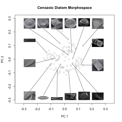
6. Choose a few (graphically, seven might be a good number) to represent around the edges of the PCO plot.
7. Produce diagrams/drawings to represent those character states visually next to the subplots for those characters.
8. Amend the drawShape() function to also reflect pattern center and raphe presence/absence (or find alternative solution).
9. Try a 2*2D morphospace plot and see if it (axes 2 and 3, or 1 and 3) looks appreciably different.
10. Construct the 2-D (or 2*2D) morphospace plot with the character plots and diagrams around the margin.
11. Write a description of the morphospace plot and how it was made.
12. Figure out how to get the topology of one of the diatom phylogenies (Sorhannus, Medlin, or Kooistra) coded so I can plot it in R.
13. Select the genera from the tree that are also in my morphospace, and plot a phylogeny of just those in R.
14. Color the taxa of the phylogeny by clade.
15. Highlight the same colors on a 2D or 2*2D morphospace plot.
16. Make a combined plot of phylogeny and PCO.
17. Describe the phylogeny vs. PCO plot, how it was made, and what it shows.
18. Finalize the morphospace through time plot.
19. Obtain genetic data from Sorhannus, Medlin.
20. Calculate genetic distances from sequence alignments.
21. Compare results of different distance algorithms.
22. Check and make sure the distance matrix from R matches that from MEGA (if it can be made to work).
23. Plot genetic distance vs. morphological distance for Sorhannus data.
24. Plot genetic distance vs. morphological distance for Medlin data.
25. Describe the genetic distance plots and what it shows, and how it was made.
26. Implement the bootstrapping algorithm that Foote used for his average pairwise distance calculations.
27. Plot average pairwise distances—decide if for smaller time bins (per 2-myr?) or per stage.
28. Find an algorithm for calculating alpha-shapes.
29. Find a good alpha-value (it’s an arbitrary choice, right?).
30. Calculate alpha shape volumes for each time bin.
31. Repeat for convex hull volumes, which should be doable with the same algorithm.
32. Implement SQ subsampling for diversity in R.
33. Perform SQ subsampling on diatom data.
34. Perform rarefaction subsampling on diatom data.
35. Generate a big plot comparing various diversity measures with disparity measures.
36. Write about how that plot was made.
37. Write about what that plot shows.
38. Go over the list of characters and pick some that might have biological meaning (linkage, defense, etc.)
39. Make plots of absolute/relative abundance of those characters through time.
40. Make big plot combining the trends in those characters through time.
41. Describe what those plots show.
42. Write code that will find the occurrence of characters (rather than genera) in a time bin.
43. Sort the characters by first appearance.
44. Make a plot of characters through time (range-through, presumably).
45. Describe what that plot shows—highlight some of the more interesting first appearances and, if applicable, disappearances.
46. Link the diversity rarefaction algorithms (see above) to the various disparity calculations (see above).
47. Read up in Foote’s paper if he did anything else fancy with subsampling.
48. Make a plot showing the effect of subsampling on the various disparity measures through time.
49. Describe how the subsampling of disparity measures was done.
50. Describe what the subsampling of disparity measures shows.

Phew! A little overwhelming… but it’s better to have it written out in a list I can check off item by item than having that shit all swirling around in my head.

Amazingly, in the course of the day, I got replies from both Sorhannus and Medlin, and Sorhannus had even sent his data by the evening. I spent Friday evening and most of Saturday working on the data, calculating genetic distances by various means and them correlating them with the morphological distances from my d matrix. By the end of Saturday I had a distance-vs-distance plot ready:

This is pretty interesting, because it’s not at all what I expected. I mean, I wasn’t expecting a perfect correlation or anything, but provided I haven’t fucked anything major up, there’s basically no correlation whatsoever between the morphological distances and the molecular distances. Wowzers! That either means morphological evolution is totally decoupled from molecular evolution (at least as measure by SSU rRNA sequences), or my morphospace is shit. Either way, an interesting result. I was also able to show that the choice of distance measure doesn’t have a huge effect on the strength of the correlation—the R-squared value is never much more than 0.05, is almost the same for most distance measures except for GG95 and TV, i.e. the Galtier and Gouy (1995) model where the G+C content may change through time and different rates are assumed for transitons and transversions, and TV, which is the number of transversions (if I decide to write that in the paper, I’ll have to understand what it means, first—I currently have no clue).

Well, I’d say it’s been a successful Saturday. I think I’ve accomplished something, both in getting a first result on the comparison of morphology to phylogeny, even though I don’t understand it, and in laying out a roadmap for the rest of the month. Even though it’s a long way to go, I now have a set of directions I can follow ‘blindly’ without having to worry too much at any time what my next task is supposed to be. Yay me. Now on to take a well-deserved few hours off.

This week has been really, really hard. And I put it down to the overwhelmingness of the job search. My calendar has been utterly overwhelmed with career events and talks, I’ve spent two nights after work at recruiting events or related talks, I’ve had at least one or two talks or events to go to each day, and my head freaking hurts from all of the information coming in, and the conflicted emotions it’s causing.

I haven’t gotten jack shit done in research. Good example: today. I was up late last night after attending a recruitment event for Innosight at the Charles Hotel, and had a terrible time getting out of bed in the morning. I made it in to work just in time for the JAWG meeting at 10, which lasted until noon. Then I grabbed some lunch. Now I have a pitifully short period of time before the next presentation I should go to, at 2:30, which—if the last week is a guide—will be utterly unproductive, because my head is spinning with job-hunting indecision, anxiety, and uncertainty. It takes time to go from practicing your answers to interview questions about your leadership qualities, or digesting a potential employer’s presentation and interaction, to figuring out how to plot individual character states on a morphospace in R. These activities reside in very different spheres, and it is exhausting beyond belief to try, daily, to go back and forth between them.

Fuck, fuck, fuck. I have gotten no research work done in the last week, and almost none in the last two. I’ve gathered an assload of impressions and information about consulting, business culture, the range of employment out there, Inkling, interviewing, resumes, business model innovation theory, and how to prepare for case interviews. But I’m feeling more overwhelmed than ever, and am coming ever closer to packing it in and giving up on the job search for this round. I need to focus on the PhD to get it done. It will not get done at this rate. I will find something, anything, to feed, clothe, and shelter myself for a year once I am done. I want to focus on this. I want to get it done. And then I want a sabbatical, some time off of serious career brain work, to figure out my next steps. It can’t all happen at the same time. It’s too much pressure and if I keep subjecting myself to it I’m just going to crack.

It somehow took me most of the day, and most of non-wasted time Friday (what the hell did I do yesterday?), but I finally managed to annotate my PCO plot with images of diatoms. And, I did this in the least efficient yet most elegant way possible (by a completely flexible and extensible R script that will now automatically draft figures like this for any given list and number of taxon names, provided there are similarly named JPEG files in the designated image folder). Woot.

In other exciting news, finally managed to follow up on a career event in a timely fashion—sent off emails to the recruiter and a consultant from InnoSight, whom I had met at a career thing on Friday (one of three events I went to that day…). The company seemed a little more reasonable in terms of their work ethic/hours/travel schedule, so I thought it worth at least continuing the conversation to the next step. It is taking me a while, but it seems that I am learning, and getting better at this whole “networking” and “job-hunting” endeavor.

Anyhow. In five minutes it’s time for the next event to start—a presentation from the barf-inducing Bain & Co about case interviews. But, I’m tired of working and have some time to bridge before Kati comes back across the river, and I might as well learn something about the interview process if I am going to go through it with some company eventually.

A thoroughly enjoyable, though exhausting, weekend with the in-laws—fantastic to get the mind off work, but overwhelming to come back to it and realize just how much there is still to be done. Did some emails, some OmniFocus-reviewing to get the career tasks lined up and out of my head for the week, and then promptly spent a good hour procrastiwebbing away as a surge of anxiety hit. Oy vey! Having all this job hunting/career exploring stuff going on is wreaking absolute havoc on my research productivity. It’s a good experience, I’m learning a lot (including, increasingly, what I don’t want to do—cf. Friday’s consulting nanocase about the Brookline Library). But man, it’s taking it out of me. An book review on NPR.com today I think sums up quite nicely the source of tension and anxiety…

Anywho, I eventually rallied and dug up a few Mike Foote papers that I hoped would inspire me to figure out what sort of analyses to do with my morphospace. Before delving into that, though, since I had promised Andy a meeting today, I tried to finish off the code that would place raster images of my diatom genera alongside the morphospace plot to show their morphology, a task that I’d started on Friday.

Finally got out of the house early enough to fit in a swim, then met Michael Lesley for a brief breakfast chat, and eventually settled down to work. It was a pretty nervous morning, as the impending titular event of the day approached, and I didn’t have much of a brain for my morphospace work.

An email came in about next weeks’ career events, and I got very distracted doing a bit of background research on the companies attending the Consulting Boutique Night—an opportunity, I thought, to meet some people who were not part of the Fortune 500/big 5 consulting world. Found it pretty interesting to see the stark differences in language used on their websites among the 17 firms listed as attending. The “about us” descriptions were almost non-overlapping—for some, it’s all about value maximization and other finance/management-speak garbage, others seemed to focus on totally different things in their self-descriptions. Altman-Vilandrie focuses on just a few industries, that happen to be ones that sound kind of interesting: communications, media, clean tech and related technology. Dalberg says their goal is to raise living standards in developing countries and solve global challenges. Innosight seems to be all about innovation, based on the “disruptive technology” idea from HBS prof Clay Christensen, who founded the company (their employee profiles were definitely more interesting than just B-school types—they seem to have a lot of interesting people on their staff with a variety of backgrounds); best of all, they’re in Boston. The others were obviously not for me—any firm that lists “financial services”, “business services”, or “private equity” under their specialties is automatically off the list for me. The Greatest Good sounded like they might be cool, from their name, but turned out to be an economist-haven. No, thanks. I don’t think I’d be happy working for the author of Freakonomics (literally), throwing rational utility-maximization dogma at any and every problem in the world.

Settled down at Darwin’s this morning to stay out of the rain and away from the office, where that uncertain new officemate awaits (or might await, who knows). Caught up on scheduling my week, decided not to go to the graduate consulting club this evening (it’s just not me—I don’t want to be on campus for an event starting at 7:30 pm unless it’s something I’m really passionate about, and I guess consulting case prep just isn’t one of those things). Decided that since Google is the one employer coming to the career fair on Friday that I’m seriously interested in working for, I’d look into what branches of the business I’d actually be interested in.

They have a /edu section to their website, which touts a variety of products and applications but did not give me the sense that there was an actual business unit dedicated to education or education-specific technology. In a blog post about their Boston office there were, likewise, several educationy-related activities outlined, but they mostly seemed to be something the resident engineers and programmers did on the side, rather than as their main job function. Read through all the job postings in Boston—it seems what they’re looking for here is experienced salespeople for management positions, or computer programmers. That’s not me. Not clear where or how their google.org type of jobs actually exist, and whether there are actually any positions dedicated in an educational direction. Hmmm.

The exploration left me a little bit disillusioned, although it’s always possible to take the sort of approach that Evan suggested, those many months ago—choose the company, and decide what position they need to create for you… I’ll have a chat to the Google person on Friday and try to scope them out a little.

Eventually did a bit of work, though interrupted by a horror story from second year Steven Jaret (who just failed his quals) and another rub-it-in defense by a fellow G6, Jenny. Found that, though time, there is basically no pattern in the expansion of morphospace. Fuck a duck. Yucky, yucky, yuck. Makes me sick. Here’s the depressing plot:

Well, that’s not good. I’m going home. What a steaming pile of dung.

Had a very reassuring meeting with Andy this morning, who was very excited about the morphospace results I showed him and appeared to be very optimistic about their potential to form both a “good thesis chapter and a good paper”. We also discussed how to proceed with the book chapters the PlanktonTech Germans had requested, and each (later on in the day) submitted an outline for a chapter to them. Done.

Buoyed by that morning conversation, I went along to the Job Acceleration Workgroup meeting, which was mostly about “elevator pitches” (not very useful for me, as I don’t really know what I’m angling for yet, but illuminating to see how difficult it is) and the schedule for the weeks ahead. Crucially, I had a great conversation on the way out with a fellow PhDer who was also interested in consulting but has become quite disillusioned with the idea; it was nice to make contact with a kindred spirit.

Later in the afternoon, I returned to R to press ahead with the morphospace and address some of the major problems I ran into late yesterday. Mainly these centered on the genus names in Neptune not matching the genus names in my morphospace. I discovered, and fixed, further errors in Neptune:

1. Aulacoseira is misspelled as Aulacosira in Neptune.
2. According to my notes Bolli says it’s Lisitzinia after all, so I changed it back.

Unfortunately, something with the factors was going very wrong, and I now have to go back over what I did yesterday and start again. I had also accidentally merged Liriogramma into Asteromphalus, which means the former didn’t come up with any matches in Neptune when called from the matrix. Anyway, I’m not sure I’ve been renaming things properly, so I need to go back and start that whole thing over…

For Mediaria, Campyloneis, and Stictodiscus, I also had two entries each in the matrix, to distinguish between different valve morphologies. This doesn’t work with the Neptune integration, since I can only have a 1-1 mapping, so I took the triangular form of Stictodiscus and the raphe valve of the other two and threw the other lines out of the matrix for the reanalysis. I just removed those lines out of the .txt file which I call from R (they’re still in the .numbers file for future analysis).

The solution to the renaming problem was simple but profound (aren’t they always?): my genus names were being stored in the data frame as factors, so trying to change the value of an entry or set of entries to a string not found in the factor levels caused a problem. The solution was simply to read in the data frame from file using the read.table option as.is=TRUE, which suppresses converting strings to factors. Less memory-efficient, but appropriate.

Fixed the names, but since re-running the distance matrix was going to take some time, decided to head home at 5:20 and let it run there.

Monday was a pretty devastating day—better documented in DSA notes than I will here, but leaving me reeling on Tuesday. By the end of the day, I felt much better, having talked it through with Kati and Beau; I came to the point where the realization that I have a working identity, shaping and forming, and that it doesn’t include surrounding myself with people who think labor unions are an undesirable thing to be associated with.

I took most of Wednesday, too, to recover, getting some exercise in the morning (it turns out that having a strict schedule is the best way to accomplish this, and I’m glad to report that I’m back on one!) and going to see a couple of 1st-year talks in the afternoon, motivated by the last vestiges of collegiality left in this graduate student.

This morning, however, anxiety levels surged again. There was an email from PlanktonTech informing members of the structure of the forthcoming Springer Verlag book associated with the project—including two (!) chapters written by me. Spoke briefly to Andy about this, who agreed to take the lead on one of the two, but wanted an outline by tomorrow, by which time the Germans had requested a first structural draft. Then, there was an email from Dave Lazarus, telling me about his wonderful new project that is essentially my diatom diversity project, except for radiolarians, though he appears to also plan to include diversity calculations for diatoms. He is presenting the results with his PhD student (I didn’t even know he had one) at the TMS (micropalaeo society) meeting in France next week. So, it seems I am scooped, again, in a way. Fantastico.

To add dung to the steaming pile, there was a reminder from OCS that the sign-up deadline for the job acceleration workgroup was tomorrow, so I had some thinking to do this morning. Do I take my visceral response from Monday at face value, and drop out of the on-campus recruitment experience altogether? I decided that I would take part after all, go to events and talk to people, eat some free food, but not apply for anything that isn’t 100% convincing. There are sure to be one or two companies that will interest me—notably Google—and it can’t hurt to get a bit more experience in the process. So I spent some time re-shaping my resumé to incorporate Laura’s feedback from Monday, and submitted it to Amy to sign up for the workgroup. Crucially, though, I didn’t change the RSMU section. I was president of an organization called “Royal School of Mines Union”, and I’m not going to lie about it. If I had worked at the Microsoft Corporation or the RAND Corporation I wouldn’t doctor my resumé and say I had been a member of the “Microsoft Collective” or the “RAND Organization” if I was applying for a left-leaning job. On the one hand, it just seems idiotic to lie in that way. On the other hand, keeping that line on my resumé is, I think, a good canary for my own happiness in the application process. If a company is going to take offense at the word “Union”, then they’re probably not a good fit for me. End of story.

Maybe this seems like a small and inconsequential thing, but it carries some symbolism for me—a commitment that I’m going to be true to my values, to my gut feelings, and to the pursuit of a kind of work that feels genuine. And I think as long as I keep that in the forefront of my mind, stay true and honest to myself, I’m OK to go ahead and milk the job-hunting/on-campus recruitment program for what it’s worth.

The non-work portion of my worries finally out of the immediate way, I settled down to trying to get some actual research done as well, in preparation for meeting with Andy tomorrow morning. Loaded the Neptune database up in R and created a new field, N$Genus, containing only the genus name (strsplit’d out from the N$Species field). Made adjustments in the dataset to reflect mistakes I discovered in the process of describing the genera:

• Bachmannocena is a silicoflagellate (leaving this in, it simply won’t be called in the plotting)
• Bacteriosira is Bacterosira misspelled
• Bruniopsis is a synonym of Neobrunia
• Calloneis is Caloneis misspelled (wow, holy shit… there are only two occurrences of this genus?! WTF?). Round also considers this to be the same as Pinnularia, but as I coded both taxa I wanted to check for consistency and keep both in there for the time being, perhaps expunge them at the end
• Charcotia is a synonym of Actinocyclus; again, left this one in the matrix to check for coding consistency, and left it in the Neptune database as well
• Denticulopsos is Denticulopsis misspelled
• Dicladia is a resting cell (leaving this in, it simply won’t be called in the plotting)
• Goniothecium is a resting cell (leaving this in, it simply won’t be called in the plotting)
• Huttonia is a synonym of Neohuttonia (again, only ONE occurrence… holy shit, that’s awful)
• Liradiscus is a resting cell (leaving this in, it simply won’t be called in the plotting)
• Liriogramma is a synonym of Asteromphalus, retained for comparison
• Lisitzinia is Lisitzina misspelled
• Macrora is incertae sedis or at best a silicoflagellate, not a diatom (leaving this in, it simply won’t be called in the plotting)
• Muelleriella and Muelleriopsis are resting cells (leaving them in, they simply won’t be called in the plotting)
• Naviculopsis is a silicoflagellate (leaving this in, it simply won’t be called in the plotting)
• Neodelphines is Neodelphineis misspelled
• Odontropis is a resting cell (leaving this in, it simply won’t be called in the plotting)
• Opephoneis is probably supposed to be Opephora
• Periptera is a resting cell (leaving this in, it simply won’t be called in the plotting)
• Pseudorocella is a synonym of Macrora and thereby not a diatom (leaving this in, it simply won’t be called in the plotting)
• Pseudostitodiscus is Pseudostictodiscus misspelled
• Pterotheca is a resting cell (leaving this in, it simply won’t be called in the plotting); Pterothecas its misspelling
  
• Raphidodiscus is Rhaphidodiscus misspelled (though Round et al. make the mistake, too)
• Screptroneis is Sceptroneis misspelled
• Simonsenella is Simonseniella misspelled
• Stephanophyxis and Stephonopyxis are Stephanopyxis misspelled
• Stichodiscus is Stictodiscus misspelled
• Thalassoithrix is Thalassiothrix misspelled

This done, I backtracked briefly to complete a plot I meant to make earlier, breaking down the morphospace into more groups. The result was pretty disappointing. Rather than showing more structure, the subgroups of the pennate and centric groups totally overlap and don’t at all occupy different areas of the space. So, that intuitive failsafe first test of the morphospace that Andy had suggested way back when,  as a response to my doubts about the project (“it has to be true, for example, that the invention of the raphe represents the invasion of a new area of morphospace”)… failed.

To close, some country song lyrics that sum up my feelings about graduate school quite nicely (via the VPhD forums):

Well, you filled up my head with so many lies.
You twisted my heart till somethin’ snapped inside.
I’d like to give it one more try,
But my give-a-damn’s busted.

Spent this morning in the first session of the Job Acceleration Work Group, learning “the secrets of the on-campus interviewing process and how to prepare efficiently”. Yikes. The array of events and things-to-do over the course of the next couple of months, and the breakneck pace at which the whole thing happens, is dizzying. I guess it’s “welcome to the business world”. Things don’t move at the academician’s snail’s pace outside of this ivory prison.

My first and highest-priority task is to get my resume together, and approved by one of the career counselors at a drop-in session early next week, and submitted to Amy to be eligible to join the JAWG. This shouldn’t be too hard, since I have a (hopefully) passable generic resume thanks to the (botched) BCG program application; and since I don’t have a clue yet what sort of jobs I’ll apply to, I can’t tailor it to any particular one yet.

I subscribed to the Office of Career Services calendar via iCal, which has suddenly transformed from a sparsely peppered to densely crowded. I joined the mailing list for the Graduate Consulting Club—I know, I know, consulting may not be the best path, but it seems prudent to familiarize myself with some of the language and culture of the business world if I’m considering interviewing for any sort of job in a private enterprise, and where better to immerse oneself in jargon and business-speak than amongst would-be consultants. I also finally (finally!) wrote the first follow-up email to the energy & environment job fair. This, shockingly, happened all the way back in  March (!!), but better late than never, I suppose.

In an effort to do at least one thing research-related before the day was out, I managed to figure out how to separate out groups of points to be plotted in the morphospace and assign them different colors (harder than one might think). But this gave me a little bit of hope, at least, that there was something to the spread of my data—since the pennate diatoms (bilaterally symmetrical things) and the centric diatoms (the others) seem to fall into sorta-separate areas… so it’s not totally garbage after all—perhaps. Here, the plot:

Spent the rest of Friday, and a good part of the weekend, putting together a resume for the BCG three-day thing. It wasn’t easy, but I was pretty pleased with the way it turned out in the end, and quite satisfied with Pages as a tool for laying it out (it really has become worlds better than Word). Now it’s a new week, and in spite of a late start (this time thanks to a toe injury I inflicted on myself on Saturday, foolishly, that impairs my ability to walk), it’s finally back to the morphospace. The clock is really ticking, too, because I have a meeting set up with Andy for Wednesday afternoon, so I damn well better have something to show him by then.

In spite of this, I had an incredibly tough time getting anything done today. My mind just wandered, wanted to be distracted. Did not want to code characters. I’m not sure what it is, but I think at some level I’m simply not enjoying the work, at all. I’m not able to get into a groove for the life of me, I am about as far from immersing myself, achieving that flow state, as I have ever been with a task. Every little distraction, every opportunity for distraction, even every opportunity for an opportunity for distraction, becomes irresistible. I am also very, very tired.

Ended up getting one, and only one, genus done today. Definitely much, much too slow… but I think I just need to rest and get back on my feet. Tomorrow will be a better day.