Siliceous and Delicious

After a weekend that was less productive than I would have hoped, I finally bit the bullet and made a start on laying out my index cards and building the structure of the papers. It’s been quite helpful so far—forcing myself to determine what conclusions I can actually make with the data and plots I have makes it clear that those are the questions I must ask at the outset, and build introductions to support.

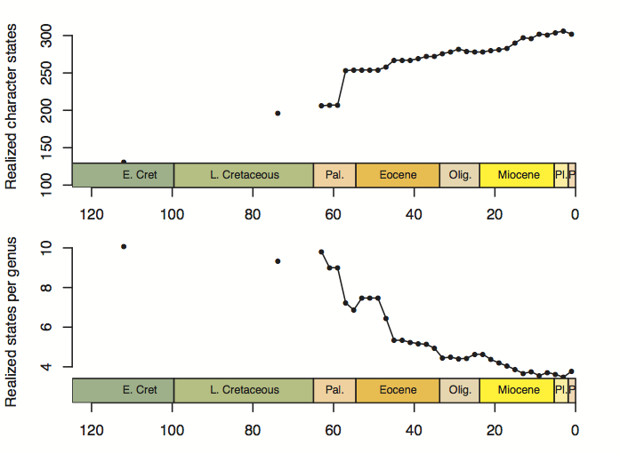
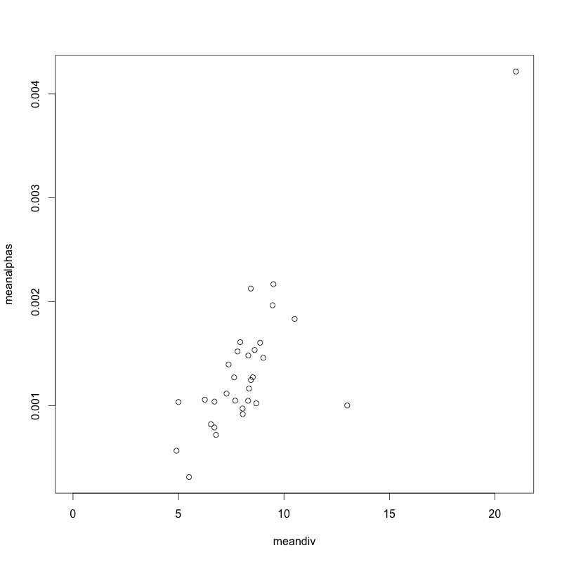
A big sticking point for me right now is the first paper. With the exception of the side-track about morphology and phylogeny, this paper is basically about “how to build a morphospace”, which isn’t really an interesting finding so much as a long methods section. The one thing I realized in doing it, and that Andy found quite interesting too, is that the choice of data culling criteria can have a pretty substantial effect on what you see, and it’s not a choice that has (to my knowledge) been addressed explicitly in prior morphospace studies. But for that to be a useful finding of the paper, I will need to actually run some analyses to show how different choices affect the outcome. Setting up the choices shouldn’t be too hard—I should think starting with the full data set as collected and then executing random (bootstrap) replicates for progressively smaller subsets of the original data is the way to go—but I’m not sure what metric I should use to show these effects. Mean pairwise distance through time? This is one of those metrics that is used a lot, but then I need to front-load a whole lot of explanation about the through-time stuff (linking the morphospace to Neptune, etc.) that I was hoping to save for the second paper, where I think this belongs.

Anyway, these are the sorts of questions I’m dealing with. I really had hoped that I was all done with analyses by this point, but I’m not sure how well the first paper will stand up on its own without a little bit of additional work. It’s really not a huge deal—it shouldn’t take more than a day to code up once I’ve decided on a metric—but choosing an output variable that captures what I’m trying to say and works with the logic and construction of the two papers is a bit of a challenge.

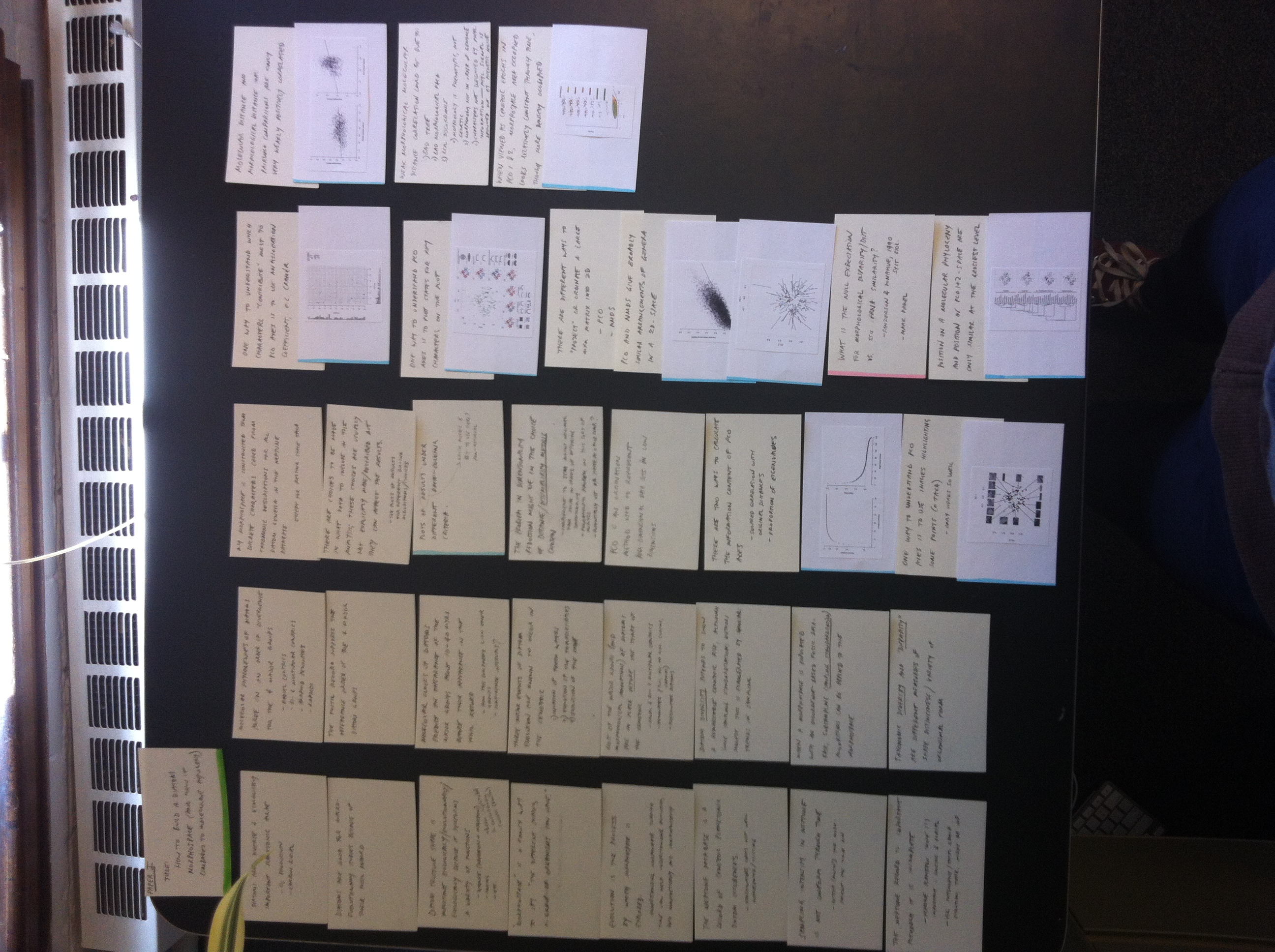
Here is what the poker table looks like, by the way:

I did also take two closer-up views of the layout for the first paper and the second paper, just in case disaster strikes in the form of wind, fire, loss, etc. You can’t be too careful at this stage.

Finally—finally!—after far too many days of (admittedly less than full steam) work , R spat out the “specific character sets through time” plot. The idea behind this was to choose a few possible adaptive roles the silica frustule plays in diatoms, and then see if character states deemed more supportive of a particular role became more common through time. For example, supposing the frustule has something to do with defense against predation, we might expect the number of genera with spines, reinforced bars and ribs, more spherical (crushing-resistant) frustules, and so forth relative to those lacking such features to increase through time.

Well, to cut to the chase—for all four functional avenues I explored with my data there is a remarkable absence of any sort of trend through time. They’re all as flat as a dead man’s ECG. Sigh. What a spectacularly poor use of my time! What a disappointment! What a surprise that the very last analysis, for which I was holding onto all of my saved-up hope, the one that was going to give sense and meaning to the whole project, turned out to be a total dud…What a joy to leave this idiotic line of inquiry behind!

Well. Now that I have all this code together (which was trickier to write than I expected), I might as well look at individual characters. Perhaps it’s my choice of characters grouped into the four character sets that is essentially causing a central-limit-theorem-like averaging because they are essentially randomly distributed trends.

Here’s what that plot looks like:

This confirms the suspicion, to an extent. Some characters do have trends, but they’re largely feeble, and by no means consistent. Together that seems to wipe out any trend in taking the average over many characters. Oh well. That’s that!

The end of last week was a bit of a struggle—the accumulated weeks of struggle combined with watching SJ and John Crowley defend (in the same day) drove the point of my stasis home with a vengeance. It was a bit of a low.

It was doubly pleasant and important, then, that the weekend was a real raiser of spirits. On Saturday Kati and I got away for the day, spent a very relaxing morning talking at Darwin’s, and then a restorative afternoon walking through Maudslay State Park in Newburyport. It gave us the chance to finally spend the sort of quality, pair-bonding, unstructured and carefree time together that I had hoped Copenhagen would provide, but was disappointed that it hadn’t. Perhaps it just needed time, but things feel markedly improved this morning.

On Sunday afternoon we spent some time with Evan and Katie (and Gavi), which was also a surprising source of motivation. Evan has an almost uncannily positive attitude to big tasks and intimidating projects at work. Perhaps it was because I came primed from a weekend of relaxing and connecting, but somehow giving my usual “no, I’m not done yet” pity party spiel this time inspired me to take a more Evan-ish, optimistic, go-gettum view of the task at hand. I am at a point where I can finish up (these first two chapters, at the very least), and what a formidable challenge. So, instead of moping, fearing, and pushing my head far into the sand until the last moment of the weekend, I actually spent Sunday evening quietly looking forward to getting to work and moving forward. I programmed the coffee maker before bed and felt rested and ready to go this morning.

Anyway, this is all a long preamble, but the bottom line is that I am working at Darwin’s today feeling qualitatively different than I have for the past few months—since the big push started petering out in March.

It’s been a slow trickle coming back from Denmark. I have been writing a bit more in my document (see the results here), but then decided that a better way to go was to write topic sentences for paragraphs/main points out onto index cards to be subsequently arranged into a logical order, the first attempts at which I have also been sketching out (in an actual notebook, with an actual pencil).

This afternoon I finally bit the bullet, booted up R, and started the final couple of analyses and plots. I think I’d been holding onto them as a last resort of “I know what I’m doing” type of tasks before the truly gaping maw of writeup uncertainty. That last resort is now dwindling. Here is the plot for the number of realized character states, including a panel standardized by the number of genera in each time bin:

The number of realized states goes up, unsurprisingly. This agrees with the PCO volume metrics (convex hull/alpha shape volume). When divided by the number of genera, though, the realized states go down—meaning each genus contributes less “raw” morphospace individually as time goes on. This I think reflects the same thing as the mean pairwise distance plot, which also goes down through time (at least a bit)—more and more taxa are being packed into the occupied volume of morphospace, and it’s happening more quickly than the expansion of morphospace itself.

One of the remaining plots I had on my list to do was the “number of realized pairwise character combinations” through time, mostly because I had read it used in a few different places (including the review by Ciampiglio, the review by Erwin, and at least one of the Foote papers), but I had not understood what it meant. I spent some time yesterday reading about it, and I think I get it now. But I am not sure if I want to bother to do it.

Here’s my best stab at explaining what the “realized pairwise character combinations” are. First, it helps to think about what a morphospace of discrete characters looks like, or at least can be thought of. Let’s start in lower dimensions. In 2D, we can think of a morphospace with just two characters, say color (red, green, or blue) and outline (square, circle, or triangle). This could look like a 2D grid, or matrix, where each square can be occupied or unoccupied by an organism.

-          Red   Green   Blue

Square      X              X

Circle             X

Triangle                   X

In this example, we have red and blue squares, but no green squares, blue triangles but no red circles, and so on. Now we have two characters with three states each, and six character states in total. But there are nine possible pairwise character combinations. Let’s add another character. If we add limbs to this—with states one or two—we get an additional dimension, or two “layers” of these nine combinations for a total of eighteen possible configurations of organisms. The more dimensions (characters) we add, the more sparsely occupied the morphospace will be for any given number of organisms. For example, in our 2D space we could realize all possible morphologies with 9 organisms, if they were all different; for the 3D space we would need 18. Add another character with four states, say, and now we need 72… so as you can see for a large space such as mine, the number of possible combinations becomes huge.

In my case, I’m not sure what it is exactly, but assuming an average of 3 states per character and 123 characters, that’s 3^123, or 5 x 10^58. That’s somewhere between the estimated number of stars (10^23) and the number of atoms (10^80) in the universe. So, with about 140 taxa, a very sparsely populated space. So comparing how the space in its full dimensionality fills up through time doesn’t make much sense—it’s going to go from being basically empty to being basically empty.

So what to do?

What I’ve done in the graphs above is to collapse that hyperdimensional space into just one dimension—think of it as a linear row of boxes, each box representing a character state, either filled or unfilled. How many boxes are filled through time? For the toy example above, it would look something like this:

Red   Green  Blue  Square  Circle  Triangle  One limb  Two limbs

X       X      X     X       X        X         X

Clearly, this is an easier space to fill! In the toy example, I’ve assumed there are no two-limbed things, only one-limbed things… In any case, that’s the idea for the plots I posted above. Now, here comes the conceptual jump for the pairwise character combinations!

Made this plot, following on from the plots showing average list length through time and average convex hull volume per list through time. It struck me that they looked similar, and indeed, when time is taken out of the equation and one is plotted against the other, it seems indeed that the major control on morphospace occupied by a list is the diversity of that list (at least when viewed on average per time bin).

What does this mean? Well, in the most conservative (and perhaps cynical) interpretation, I would read this to mean that morphospace is pretty well constant over time. Some lists are longer than others, perhaps because of the choice of what taxa to list for a particular section, or perhaps because there were simply fewer taxa present in the section. But the more taxa are found, the more morphospace is occupied. The two outliers are, of course, the Cretaceous samples (data collected according to very different rules), the rest fall on a pretty tight trendline.

Took the day off to see Tufte do his thing. It was cool. I liked the idea of making graphics about the content, and putting everything in service of the cognitive task at hand—of making every aspect of the display support the intellectual activity the display is trying to accomplish. At many points along the way I reflected on what this means my morphospace project. In some ways, a helpful reflection. In other ways, reinforcing my crippling stuckness. There’s nothing I can accomplish with a good figure if I don’t know what I’m trying to say with that figure.

The metaphor is the map. Make the graphic as clear and uncluttered and minimal as a map. But, how can you make a map if you don’t know where you’re going?

“The best good design can do is not to get in the way.” I liked that thought. But it scared me a bit, too, because in some ways I feel like well-designed figures is all I have in this project. What I’m lacking is the spine to back it up.

The sun is out, it’s forecast to be in the 70s today and up to 80 tomorrow. It’s the first day of spring. I’m sitting outside Darwin’s in a t-shrt, it feels wonderfully fresh and warm, and yet there’s something holding me back from really enjoying it. What, oh what could that be…

I feel totally paralyzed, still, by that question Zoe asked on Friday. What can you say about your results? I just don’t know. What are the two points do I want to make? What am I trying to say? What question is this morphospace project answering? Fuck.

Beau helped tremendously in DSA today. Somehow, talking it all through crystallized for me that there’s only one way out, and that’s through me. The help is going to come from nowhere, so I need to muscle my own way through it. Asking for help, being humble and self-critical and loyal to the truth is going to get me nowhere. I’ve had the best results in the past when I’ve been confident, self-assured, argued by advocacy and basically played the part of the blowhard. That’s just what I’ll have to do to get through this.

Motivation is at a new low. I just can’t seem to summon the energy to do any work. I am just dispirited.

It took me a long time to get going, once again, and I spent the morning catching up on DSA posts for last week. Scott Edwards got back to me by email and I tracked him down in the afternoon for a chat about molecular vs. morphological distances. He was incredibly nice—just a really friendly guy—and I did get one or two references out of him. But in general I found it quite hard to get much out of him that was directly helpful. What I had been hoping for was context and explanation of the plots I’d made, basically a sense of what that distance comparison would look like for other groups of organisms, and whether my plot is expected or unexpected. Instead, I found that he seemed most interested in advising me to do other analyses with the data I have—mainly studying the evolution of characters on the tree, relating morphological change to speciation events, for example, seeing if disparity grows anagenetically or cladogenetically, and so forth. These are of course really interesting questions, but they’re a lot of extra work and analysis that I don’t think I have to the time to do. There just seemed to be an almost unbridgeable gulf between my approach (focused on morphology alone, making comparisons to phylogeny and diversity) and his approach, which appeared to be entirely phylogenetically focused.

Went straight to MIT for my 10:30 meeting with Zoe and Andrew. They were good and active listeners, and had a lot of both nice and constructive things to say, but at the end of the day it still left me dispirited. Firstly because I realized, as I have done oh so many times, over and over again, that I am the only one who can figure this out, and (almost) every time I ask for help, I realize that I have to answer the most difficult questions myself. And secondly because we ended up talking, inevitably, about the future, what I was going to do next, whether I wanted to a postdoc or not, and so on, a conversation that I try to avoid because always leaves me completely unsettled and usually depressed.

One useful piece of the conversation, though also source of my disappointment, was the point Zoe made that I needed to know what I wanted to say before I wrote the papers. What did you find? What are you trying to say? What question is this paper answering? These are the matters about which I’ve been plugging my ears yet Zoe is absolutely correct in asking these as prerequisites—and, sadly, there is probably justification in her incredulous eyebrow-raise when I mentioned that I wanted to get the first paper finished by the time I head to Denmark at the beginning of April. This is so much harder than I thought it would be.

Anyway, she was no help whatsoever on actually answering these questions for me, but she and Andrew did make a lot of other useful and helpful remarks, including these I’ve chosen to highlight as relevant and actionable:

1. If you divide morphospace occupancy (alpha volume) by the number of species for each time bin, is that a way of standardizing for sampling? [Note: maybe not, but it would give an interesting other measure of per-species morphospace occupancy, a sort of analogue of mean pairwise distance.]
2. Can you circumvent the sampling problem by plotting the morphospace occupancy of individual lists/sites for each time bin (i.e. alpha morphological diversity through time)? I think this is both interesting and helpful, and allows a discussion of the analogy of alpha and beta and gamma diversity with disparity through time, which I’m not sure has been done before (well, it probably has, but I don’t know about it).
3. What about plotting the number of realized character states through time? Wouldn’t that be a good measure? [Note: I think this is similar to the metric of ‘realized pairwise character combinations’ or whatever it’s called from the disparity literature.]
4. Zoe and Andrew both made a bit of a fuss about how my dataset isn’t independent of phylogeny because I used genera, which are defined morphologically, as the basis for my study. I’m not sure I understand why this is a problem, other than that there is sure a lot of intrageneric morphological variation that is not captured by my morphospace. The way around it of course would be to score individuals in samples (without necessarily even naming them or assigning them to a genus), and do this for a large number of samples through time, but of course that’s an utterly unrealistic effort and the mere thought of it makes me want to throw up.
5. Can you plot mean pairwise molecular distance through time? Using Neptune to time-resolve the pairwise distances from the Sorhannus tree. Would it look different from pairwise morphological distance?
6. Zoe also suggested what I’ve been wanting to do for a while now, but haven’t yet—i.e. looking directly at particular characters in the data set. When I pressed her to suggest ones that would be interesting to look at, she came up with a list that was (actually  reassuringly) similar to what I’ve had in mind: characters related to chain formation, chain formation characters resolved by silicification (i.e. are they using less silicified structures through time to achieve chain formation?), pore size through time, velum presence/absence through time (this relating to the viral/pathogen defense hypothesis), predation characters, sphericity (SA:V ratio, for both strength, nutrient uptake) and possibly labiate processes/raphes if anything meaningful could be gleaned about their homology from patterns seen in the morphospace through time.
7. With regard to my difficulty in thinking about the chain formation vs. predation characters, Zoe was encouraging—her take was that this is a real problem and rather than ignoring it I should simply write about how it is difficult to disentangle whether spines are for one or for the other, and just describe what my observations would mean for either hypothesis.
8. She also suggested going through my list of all characters and brainstorming creatively about what each one could mean functionally, keeping in mind what the main important factors are (which is another difficulty, but never mind—I wrote down “predators, sinking…” in my notes).
9. In the morphospace occupation density plot, she wanted to know what the morphotypes are that are disproportionately represented—a good question I should answer if I am going to put that plot in the paper.
10. Finally—what two things can you say about your data? This is the crux, really. I need to figure out what I can say about the data, and then shape my paper based on that.

Altogether a challenging, exhausting day. Some things gained, but much confidence lost. It just feels like there is an eternally long way left to go, and the path ahead just doesn’t seem to get shorter.

Zoiks. Best not to think about it too much.

In spite of being on the mend, still felt pretty grotty and exhausted in the morning, and consequently didn’t arrive at the office until well after 10 am. Fired off emails to Scott Edwards and Zoe—setting up a meeting with the latter for Friday morning (the former is out of the office for a while).

In the afternoon, helped Wil with a stats problem. He was trying to do a nonlinear regression in Excel (a nightmare), and I was able to figure it out in R in less than an hour. I was quite proud of myself and felt very useful—once again, it’s proving an invaluable skill to have under my belt. I did hesitate for a moment, thinking I shouldn’t take more time away from work, but since I was mostly stewing about how to write up my chapters, I figured I wasn’t that productive anyway, and that model fitting was something I really ought to know how to do in R. I promised myself I’d take no longer than an hour and then give up.  That turned out to be ample time.

I spent the rest of the working day reading two of Mike Foote’s papers, one on “Rarefaction analysis of morphological and taxonomic diversity”, which I ended up not concentrating on all too deeply, and the other on the Paleozoic crinoid morphospace, which I read with much more attention than I had given it before. Some thoughts:

• The rarefaction paper does classical rarefaction, (none of the fancier Alroy algorithms, which I suppose post-date that paper); what’s more, it rarefies by species, not by occurrence—because of course Foote isn’t working off of an occurrence-level PBDB type database. This is of course good news for me—I think my study might be (?) the first time someone’s actually populating a morphospace with occurrence-level data in the time dimension. That allows me to subsample/rarefy by occurrence.
• The 1995 crinoid morphospace paper is full of cross-references to other Foote papers on the crinoid morphospace. Basically, his crinoid morphospace project is a ~5-paper monster split into bits. That makes it really, really hard to read—tricky to understand one without having read all the others. I realized in the reading that I am veering into that direction with my paper, and it’s something I’d prefer to avoid. What’s the point of doing all that detailed work if nobody’s going to understand it because it’s presented in a scattered and opaque manner?
• His work is almost all at the abstract, morphospace/disparity/diversity meta-level. Rarely does biology, function, or phylogeny enter into the discussion. This is, on the one hand, heartening—if he can do it, so can I. But it’s also unsatisfying.
• Where he does touch on biology: early on, he sets up the idea of “morphological constraint” in crinoids, i.e. the idea that crinoids early on hit some sort of intrinsic limit on morphological diversity, and the subsequently just evolve about in a constrained space. This acts as a straw man of sorts for developing his arcane mathematical manipulations of the morphospace data.
• In toto, I’m not entirely enamored of using Foote’s paper(s) as a model for my own.