Siliceous and Delicious

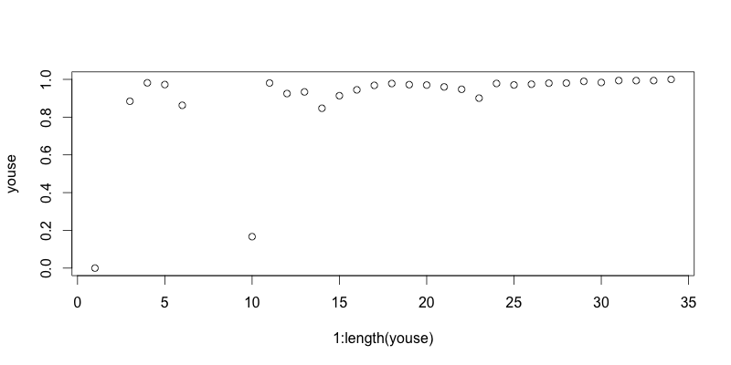
The weekend was not super-productive, although I did put in some time on both days. I was pretty exhausted on Saturday after spending the morning volunteering at the museum, and spent some time napping at Pierre and Nicole’s while Kati babysat Alexandre. In any case I managed to spend several hours over the course of the rest of the weekend tidying up the subsampled plot so I’m now satisfied with the way it looks:

This done, I moved on to tackling the next task, which is to try and answer Andy’s (legitimate) question about which characters are actually responsible for changes in morphospace occupancy. To accomplish this, I wrote code that compares the taxa in the alpha volumes of adjacent time bins and finds the taxa in the new, expanded volume of the younger time bin (i.e. those taxa that fall outside of the volume of the older time bin). The code then compares the character states of those taxa with the taxa in the older time bin and identifies which character states are new. Those character states are responsible for the expansion of morphospace volume (at least in three dimensions).

This new chunk of code returns lists of character states for each time bin, which is of course a little obscure, being a list of numbers, and requires a bit of look-up work. Here, then, is a summary of the character states that are responsible for adding alpha volume in each time bin. (This took a bit of time, too, because I decided it was too laborious to look up each of the character descriptions, so I wrote a script to call up the appropriate line of description from the text file containing the character and state descriptions).

• Late Cretaceous: 68 new states outside the Early Cretaceous 3D-morphospace alpha volume (with alpha=0.11). A lot of states to look at here. Yikes. New valve outline shapes, aspect ratios, undulations, torsion, and curvature. Apex shape, heterovalvy, topographic folds, apex topography, various other characters of the apex, central depression, ornament at rim, asymmetric mantle, warts, brim, mantle pores, surface texture, central area ornament, spinules, collar. Importantly: the first sternum. Pore arrangement and size, other pore features, bullulae, pseudoseptae & ribs, apical fields, labiate processes, some sternum characters.
• Paleocene: 53 new states outside the Late Cretaceous volume. Again, a lot. Ovate valve outline, depresse aspect ratio, frustule curvature, apiculate apices, heterovalvy, valves without a mantle, crimped mantle edge, mantles without pores or with simple perforations, more costa types, rays & associated characters, non-perpendicular pore arrangement, oval and rectangular pores, alveoli, porelli, pseudonoduli, ocelli, apical pore fields in rows, wide as well as eccentric sternum. Importantly, the raphe, in various places, singly and split, with and without canal, keel, and fibulae.
• Eocene: 17 new states outside the Paleocene volume. Rhombic valve outline, curved central elevation, more costae, central area with scattered pores, central spines or tubercles, curved and spiral rows of pores, quadrate and slit-like pores, apical and annular pseudosepta, ocelluli, sigmoidal raphes, and laterally-opening raphes.
• Oligocene: 2 new states outside the Eocene volume. Naviculoid non-sternum central area, ring of tubular spines in central area. (Whoa, random—I guess these are the only things Pseudorutilaria has that weren’t there pre-Oligocene; it’s just its odd combination of all the other characters that makes it stand out. I guess.).
• Miocene: 16 new states outside the Oligocene volume. Panduriform valve outline, curved frustule, patchy pores on mantle, ridges and grooves on valve face, biseriate pores, specialized openings, quite a few invalid states*, labiate processes along sternum, sinuous raphe, straight, deflected, and bent terminal raphe fissures.
• Plio-Pleistocene: 4 new states outside the Late Cretaceous volume. Anguste late aspect ratio, sternum widening at poles, raphe around entire valve circumference, and one invalid state*.

*It was pretty shocking to see how many invalid states there were. These are, for example, a state 3 when there are only states 0, 1, and 2, or in one case a state “j”. These are obviously typos. Clearly, they’re more likely to be caught by looking at taxa in the fringes of the morphospace and by looking at characters not found in the other taxa, but it’s still kind of freak-out-ish to think how many typos and other mistakes are lurking in my dataset. Alas, I simply don’t have the time to fix these anymore. Going through the whole dataset (even the culled dataset contains 14,000 entries) is just not feasible. End of story. The mistakes have to stay in there.

Is there anything to be learned from the characters responsible for the space expansion? Nothing jumps out at me. The shift from Early to Late Cretaceous is uninteresting to me, just because there are so few taxa in the Early Cretaceous that I doubt it represents much of anything real; anyhow, the characters are mostly related to seeing pennate diatoms. In the Paleocene… I don’t know. Just seems like a random jumble of characters. Same for the other time bins really. What a pile of crap shit poop. My guess is that the morphospace is just basically meaningless, so the characters responsible for these volume gains are essentially random.

So what remains to be done now? I have not, as promised in my to-dos for the week, spent the requisite time on my thesis document, writing, so that should probably be my next task for today, if only briefly, so that I don’t lose touch completely again. Got a couple of paragraphs on the morphological vs. molecular distances written up. Slow like treacle, but it’s coming along.

Another weekend away from work, and no, it doesn’t feel great. Somehow it just happened. Fuck.

Anyway. I’m trying to figure out how to implement Alroy’s SQ algorithm. On Friday, I couldn’t get his website to work (where he had posted the R code), but he replied on Saturday with the fixed link, and so I’m now sitting (at Darwin’s again) reading through his code and trying to understand how it works. I wish I could see it in action with an example data set, because I’m not entirely sure what sort of data the function actually takes (while his documentation is much better than the code junk I got from Rabosky, it still leaves much to be desired). Is it just counts of taxon occurrences? If so, i.e. if the function doesn’t identify what particular taxa are in the subsample, this is going to make the proposed exercise of subsampling the morphospace very difficult indeed. Well. It’ll require rewriting the function.

From a little bit more reading and some monkeying around with the code (i.e. loading the function in R and passing some sample data to it), I find my suspicion supported—it seems as though the function simply takes an array of numbers representing the occurrence counts of different taxa in a time bin, plus the other function parameters, and returns the average number of taxa in the appropriate sized subsample (over the requested number of trials or iterations). This does make calculating the diversity curve fairly easy, but makes it that much harder to get the morphospace to subsample.

Should I just rewrite the function for my own purposes? It doesn’t seem all that complicated, really… Aargh! I am unmoored. I don’t know what to do nor what I’m doing.  The approach I was taking in constructing my own SQS function back in the day was quite a bit different, passing the full database back and forth between functions; Alroy’s approach of just passing an array of counts seems much more efficient, probably uses way less memory and is consequently faster? Although I do lose the ability to track actual taxon names. Maybe a combination of the two would be the way to do it—instead of the full database, have the function operate on a list of names?

Started by calculating Good’s U (by the original, simple formulation) for 2-myr time bins. There is very little variation in coverage estimated in this way. Correcting for this is going to do nothing for the diversity curve:

This is kind of an important plot, because it shows that implementing the SQS, at least in the simplest way, isn’t going to do anything to correct the diatom diversity curve from Neptune. I think I know why that is, too. Good’s U is measuring how well the standing diversity of a time interval is captured in the fossil record by looking for how many singletons there are, i.e. how many taxa only show up once. The greater the proportion of singletons, the more likely you’re still missing a lot of the standing diversity. Here’s the big but, though: basically all of the Neptune data is collected in m*n taxonomic charts where the m rows represent m slides prepared from borehole samples at m depth intervals, which the poor shipboard paleontologist scans through to check for the presence/absence or abundance of n different taxa. [This is the model of data collection that Dave Lazarus talks about in that recently published paper I reviewed for him at such great length last year.] This method makes it very unlikely to have singletons. I think that’s why the Good’s U values are all so high in the plot above.

The numbers would probably go down a bit if Alroy’s correction for dominant taxa were applied—i.e., take out the most abundant species, but that doesn’t really address the problem of the data collection method being strongly biased against singletons.

What if there were another method to estimate coverage, not as vulnerable as Good’s U to the bias from the Neptune-esque method of data collection? What would that look like? I suppose it could look at how many taxa show up in only one borehole, since that’s sort of the equivalent of an ‘occurrence’ of a macrofossil taxon in PBDB. That would probably work quite well for the most recent time bins, where there are dozens of boreholes, but most of the Paleogene time bins have only a couple of boreholes at most, and so many would have a very, very low coverage by that measure (I think). It might be worth a try, I suppose.

Grrr. This is not helping me make progress with the morphospace. I feel like I’m disappearing down a rabbit hole of distractions and unforeseen complications again. What I need is to get this paper done. I need to get my figures together, so that I can get the chapter written. So that I can move on. This is what I need to keep my mind focused on. I thought it would be straightforward to add diversity subsampling to the analysis of morphospace, but maybe it’s just too difficult. Maybe there are just too many complications with implementing SQ subsampling for this sort of data to apply it “straight out of the box”, as had been the plan all along. Well, fuck.

Maybe I just need to refocus on something else for a little while to let the frustration subside, because I’m pretty well boiling with frustration and rage right now. I also need to re-run the stacked 3D morphospace plot for my new cull of data so that I can plop that into my LaTeX document. Might be just the thing to do right now.

After a late start (thanks to a late night at Pierre and Nicole’s yesterday), and part of the morning helping Beau figure out his very own PCO problem, spent the afternoon at Darwin’s East. Reading the Erwin paper on disparity brought up a handful of points:

1. There are a few other disparity measures I might consider—total variance, total range, number of unique pairwise character combinations, participation ratio—that I’m not too familiar with. He cites a paper by Ciampaglio, 2001, that I should check out.
2. Is there some way to assess whether the filling of morphospace is more rapid (or less) than would be expected if diversification filled the morphospace under some null model (say, randomly)? Can that be simulated (sort of a bootstrap/p-value for morphospace occupation)? Erwin references Foote, 1996b in the book Evolutionary Paleobiology by Jablonski, Erwin, and Lipps, Gavrilets, 1999 (“Dynamics of clade diversification…”), and Pie and Weitz, 2006 (“A null model of morphospace occupation”). The last one seems particularly relevant. Yikes! Lots of reading to do.
3. Can clades be separated out from the morphospace and their patterns of occupancy-through-time be examined individually? (My guess is that this will break down due to the degree of uncertainty of the tree topology).

Well, these are cool and interesting things to think about. Need to actually produce something now, though. I think setting up my code to produce disparity/diversity figures for different taxon sampling methods is next. I’m a little confused about exactly how I’m going to go about this, since I have two separate Neptune data files now, the original one I was working with on the diversity project, and the modified one for the morphospace project, which includes the crucial “Genus” column (with the genus name only). But, it has about 2,000 fewer entries than the full one, and I’m not quite sure why. It probably doesn’t matter though, since it’s only a third of a percent or so of all the entries in the database. Maybe I can just ignore it. Maybe it’s just the zero-age-value occurrences I took out. (Quick check: doesn’t look like it). I’m going to ignore it for the time being. [Later note: the difference is those occurrences of taxa that are in the Neptune database but not in the morphospace—i.e. genera that I didn’t code for. It’s actually quite reassuring that they only account for a third of a percent of all the occurrences.]

Another minor niggle I noticed: the genus diversity from the morphospace increases in the first few time bins of the Paleocene, while the species diversity seems to be zero until about 60 myr. That does not make sense—something’s fishy there. Need to follow up on that. Result: probably down to setting the time bins so they only start at 60 myr. Resetting the time bins to go back to 64 myr ought to fix that.

The problem I’m grappling with at the moment is that the code to calculate convex hull volumes crashes when I run it under the “in-bin” sampling model. It works fine under “range-through” sampling. I had problems with the mean pairwise distance function initially, too, because in the in-bin sampling mode supplies some time bins with zero length taxon lists (i.e. no occurrences). But I fixed that and the mpwd works fine now, but not the convex hull volumes. What gives? Reducing the range of dimensions used for convex hull volume calculation to 3D and 4D only (rather than 3D through 10D) makes it run OK—which suggests there’s some sort of problem in the higher number of dimensions. I’ll just have to keep redoing it until it breaks. It works fine to 5D and 6D. It crashes when I try to run it in 7D. Huh?

One observation that’s a possible lead is that, under in-bin sampling, the least diverse time bin has only 7 taxa. Is it possible that at least n+1 vertices are needed to calculate the hypervolume of a shape in n-space? It sort of makes sense in low dimensions—you need at least 3 points to define an area in 2-space, and you need at least 4 points in 3-space to define a volume. Maybe you need at least 8 vertices to calculate a hypervolume in 7-space. If this is true, no time bin under range-through sampling should have less than 11 genera in it. This is, in fact, true—the least diverse bin has 13 species in it. I think I’ve figured that one out!

Here, then, is the same figure as in yesterday’s post, but using the in-bin taxon sampling rather than range-through:

It looks quite a bit more variable and messy, but otherwise it’s pretty similar overall. I’m not quite sure why the alpha volumes with values >0.11 did not plot—maybe that algorithm crashed, too?! No, the results are there. Why aren’t they plotting, though? OK, problem solved—silly indexing mistake that crept in since I copy-pasted the plotting code for the alpha shape results from the code that plots the convex hull volumes. Never mind. Here’s the corrected version:

Well. Now that I’m not distracted by those missing lines, a few differences between the two sets of panels:

• Mean pairwise distance more variable using SIB
• Oligocene is peak convex hull volume in RT, while in SIB, Miocene is peak and Oligocene doesn’t stand out
• In alpha shape volume, the SIB curve is messier/noisier, but the pattern of increase with peak in the Miocene is the same
• There are hardly noticeable differences in the species diversity curves—this is a bit surprising (?)—I thought the RT looked a bit more different from the SIB based on my term paper with Charles all those many moons ago

OK. So now that this works sorta-kinda well, on to implementing the other taxon sampling methods. I already have routines in place for rarefaction and by-list, unweighted (“UW”) subsampling in my code from the diversity project. I should try and see if I can run those routines on the morphospace-modified Neptune database. Ah. But here’s a pretty major complication I hadn’t thought of. The subsampling algorithms all work by taking subsamples many times, calculating the diversity for each subsample, and then taking an average. Obviously, that average (which is what would be plotted in the bottom panel—no problem there, in theory) doesn’t have an associated set of taxon lists for each time bin. Rather, to do this properly I’d have to write a routine that generates a subsample, calculates the associated mean pairwise distances, the convex hull volumes, and the alpha volumes, and then does that a bunch of times and calculates the averages. It’s not that this is insurmountable, it’s just going to be a fair bit of work.

It also raises the question of how this subsampling should be done. Should the subsampling routine for the morphospace be run at the species level, and then the resulting pattern be showed at the genus level in the morphospace, or should the subsampling routine itself be run at the genus level? The latter would be more work, but perhaps the more “correct” thing to do? Phew, this is more complicated than I anticipated. Much, much more complicated. Since this is going to be a pretty major effort, I should probably do it only for one subsampling method, at least at first, and so since I will want to use SQ subsampling in the diversity paper, that’s probably what I ought to use here. But, I haven’t implemented the SQ algorithm for my dataset yet… Yikes…

Grasping at straws yesterday, in the safe haven of a DSA conversation, I came up with the latest desperate attempt at heaving myself out of the rut of unproductivity I’ve been languishing in over the past few weeks. It seems to have worked.

It wasn’t perfect, by any means, but it did the job—I am through my first pass of the list of Cretaceous taxa, all coded up. At (motherfucking) last. There were four taxa, however, which I skipped along the way because I wasn’t able to find any detailed descriptions of them anywhere. I need to revisit them each briefly for an (even) more in-depth search before I give up and just throw them out of the morphospace altogether. And I also need to do a little bit of tidying up of the matrix, as I’ve probably mentioned before, particularly with regard to the “linking spines” character, which is a bit of a mess right now with different character states represented by the same number but differentiated in (some) of the comments for the characters… That’ll take a good day of frustration to figure out, but it’ll be for the better in the end.

Anyway, for completeness in documentation, the “intervention” alluded to involved exiling myself to the tried-and-true motivation-boosting environment of Darwin’s, and turning off the wireless. It was successful in the sense above, in that I got shit done that I needed to do, but it was also somewhat unsuccessful, because I didn’t quite kick procrastination today, even though I worked at an infinitely greater rate of productivity than in weeks past. First, I found offline ways to procrastinate. These were much more productive than aimless surfing (I wrote about a page about the Snowball Earth idea, and made a first draft of a Pig & Penguin Design logo), but time away from work nonetheless. Second, I eventually caved and turned the wireless back on. The draw of checking emails, nytimes.com, salon.com, slate.com, xkcd.com (it’s Wednesday, for goodness’ sake) was just too great. Fortunately I probably lost no more than an hour in total to these diversions. A shameful amount for any honest working man, but compared to the untold truckloads of time I’ve wasted in the lowest of the low times in the past five and half years, it’s actually an improvement.

So, here’s to a successful day. Many more, one can hope—but in the spirit of Beau’s pep talk, this was just a day, and that’s the horizon. What can work today can work tomorrow. The same should go for me.